In my work applying machine learning technologies, finding “similar” items is one of the most common challenges that people come to my team with:

• “Can you find me the image that looks like this other image?”
• “Which webpage is similar to this webpage?”
• “Which song matches this audio clip I’ve recorded?”

To more formally define the similarity task, let’s assume we have a big database of items. Solving the this task means that when we are given a new item – let’s call it the query – our algorithm is able to locate within the database the closest or most similar items to the query.

Whether we’re dealing with pictures, audio clips, faces, documents, or DNA sequences, we can approach solving this problem using a common framework which I briefly summarize below.

Feature extraction

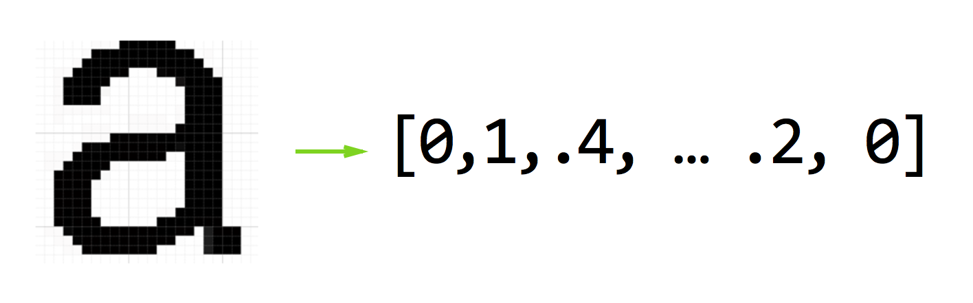
First we need to know how to “represent” each item in our data set as a series of numbers. This process is often called “feature extraction” or “feature representation”.

There is a large field of research focused on finding good feature representations for all kinds of data. And while it may not yield the most optimal results in terms of discounting noise in our data, we can take the raw signals themselves and convert them verbatim into our “feature vector” as a first step in building our similarity search engine.

So for example, if our dataset is made up of 16 x 16 gray scale images, we would take the pixel value of each row and store them as an array of 256 numbers.

Defining a similarity metric

Once we have a feature vector for every item in our dataset, we need a way of comparing one feature vector to another feature vector. If we view each feature vector as a point in some n-dimensional space, one can use the euclidean distance between two points $p$ and $q$ as a similarity metric:

Brute force similarity search

With the similarity metric and a feature extraction routine in place, we pretty much have a complete working similarity search system, albeit an efficient one. If given a query $q$, we can find the closest item to $q$ in dataset $D$ using the following routine:

def find_nearest(q, D):
    nearest_neighbor = None
    min_distance = infinity
    for p in D:
        distance = compute_distance(p, q)
        if min_distance > distance:
            min_distance = distance
            nearest_neighbor = p
    return nearest_neighbor

The approach above scales in $O(m \times n)$ time where $m$ is the number of items in our dataset $D$ and $n$ is the number of dimensions in our feature vector. So even for a modest database size of 1000 items and a feature vector of 256 dimensions, we could be computing up to 256 thousand operations with every single query!

To be continued …

In the next part of this series, we’ll take a look at using vantage point trees to see how we can more efficiently store our data set so that it’s less computationally intensive to search over.

continue to part 2 →