This is the 2nd article in a two part series on similarity search. See part 1 for an overview of the subject.

In this second installment of my series on similarity search we’ll figure out how to improve on the speed and efficiency of querying our database for nearest neighbors using a data structure known as a “vantage point tree”.

We previously used a brute force approach by computing pairwise distances between our query and all points in our dataset so that we could find items that were close to it.

Unfortunately, this technique scales in $O( \# examples \times \# features)$ time which is prohibitively expensive on even modestly sized datasets.

Kd-trees, and more recently vantage point trees (a.k.a vp-trees), have gained popularity within the machine learning community for their efficacy in reducing the computational cost of similarity search over large datasets.

For this article, we’ll focus on examining how a vp-tree works.

What is a vantage point tree and how do we construct one?

In a nutshell, a vantage point tree structure allows us to store the elements of our dataset in such a way that during query time, we can quickly exclude from examination large portions of our data without having to perform any distance computations on the elments of that excluded portions.

Let’s take a look at the basic structure of a vp-tree because it will allow us to understand how we can prune data from a search at query time.

By definition, each node in a vp-tree stores at a minimum 5 pieces of information:

1. A list of elements sampled from our dataset
2. A vantage point element chosen randomly from the list of elements above
3. A distance called mu
4. A “left” child node
5. A “right” child node

I’ll explain soon how all of these compoenents relate, but in the meantime here’s an illustration of the vp-tree concept:

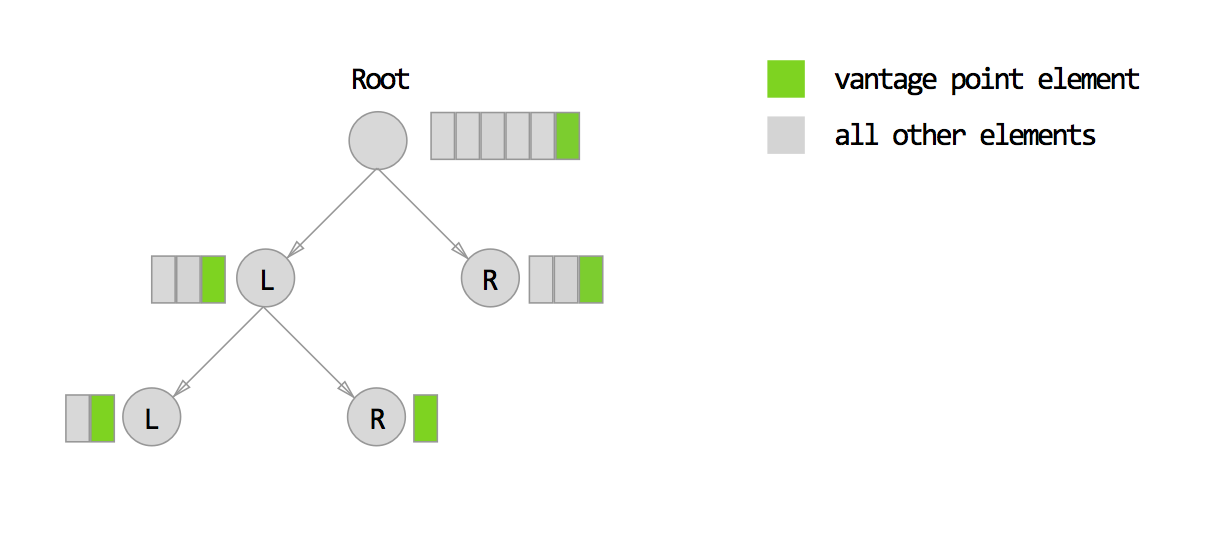
At the root node of our tree, the list of elements consists of every single item in our data set. From this list of items, we choose one element and designate it as our vangate point.

To choose $mu$, we compute the median distance between our vantage point $vp$ and all other elements $P$ in the current node .

We select all points within a distance $mu$ from the vantage point to assign elements to the left child node. And similarly, we can assign all points outside of $mu$ to the right child node.

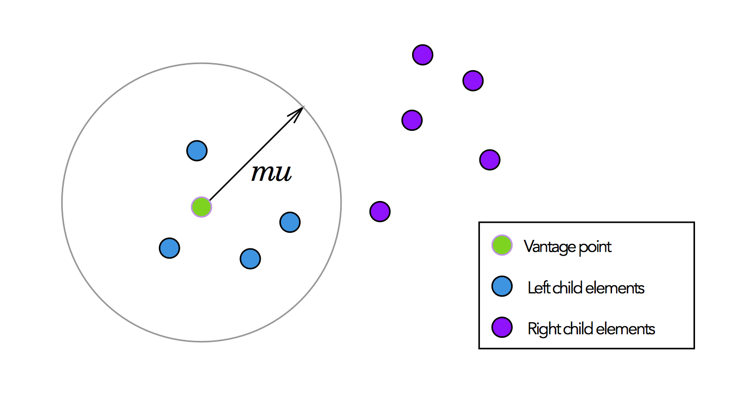
Since $mu$ is the median distance between the vantage point and all other points, this procedure effectively divides into half the elements we assign to the left and right child nodes.

Finally, to construct the rest of the tree, we recursively follow this same procedure for each child node, until there are no more elements to assign to child nodes.

Here is some pseudo code to build the tree:

class VPNode:
    elements
    left_child
    right_child
    mu

def build_vp_tree(elements):
    node = new VPNode()
    node.vp = select_random(elements)
    node.mu = median(distance(vp,e) for e in elements)
    left_elements = [e for e in elements where distance(vp, e) < mu]
    right_elements = [e for e in elements where distance(vp, e) > mu]
    node.left_child = build_vp_tree(left_elements)
    node.right_child = build_vp_tree(right_elements)
    return node

Nearest neighbor search with the vantage point tree

For a dataset encoded as a vantage point tree and a query point $q$, how can we find the closest $k$ points in our dataset without running distance computations for every single element?

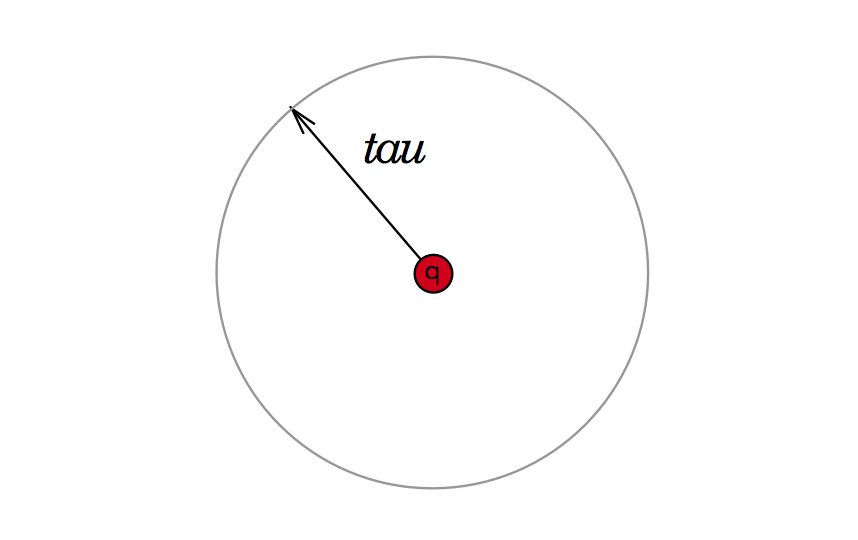
One approach we could take is to say that for every $q$ there is some threshold distance $tau$ where all of its closest $k$ neighbors are contained within this threshold. You can imagine this area as an enclsosed circle as depcited below:

There are three scenarios for how this query-tau area can relate to any node within our vantage point tree.

Pruning the left child node

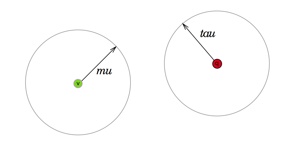
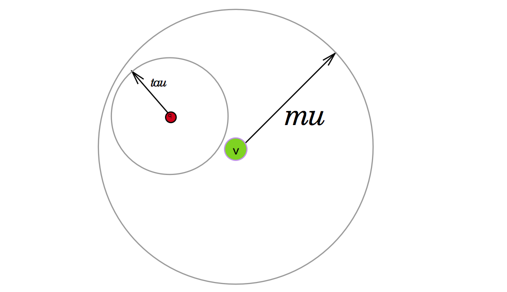
The first scenario is if the area lies completely outside of our vantage-point-mu radius as depicted below. If this is the case, we can safely assume that if we are to find $q$’s nearest neighbors we can forego looking in our node’s left child, which contains all elements within the mu radius of this vantage point.

Pruning the right child node

The next scenario is when the query-tau area lies completely inside the bounds of the vantage point’s mu-radius (see below). In this case, we can ignore all points outside of $mu$ which we had conveniently assigned to the right child node.

Worst case, we check both left and right child nodes

What happens when the query-tau area partially intersects with our node’s vantage point’s mu-radius?

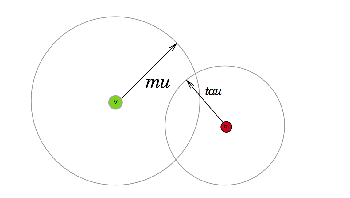
In this scenario, we can’t say whether the right or left child contains the nearest neighbors, so we have to search both nodes.

Traversing the tree to find nearest neighbors

To summarize, when the query threshold area is completely outside the bounds of our node’s vantage-point mu boundary, we can exclude or “prune” the left child node from our search space. When the query threshold is completely inside the bounds of vantage-point mu boundary, we cans safely ignore the right child node. And finally when neither is the case, we must search both left and right child nodes.

Now that we know how to behave when examining a single node, we can use this knowledge to find $q$’s nearest neighbors by recursively shrinking $tau$ as we search down the vantage point tree.

More concretely, we initialize $tau$ to be infinity. And as we traverse from the root node to each child node of the vp-tree, we set $tau$ to be equal to the lesser of the distance from $q$ to $vp$ or any previously seen $tau$.

def find_nearest_neighbors(tree, q, k):
    """
    tree = the VP tree
    k    = # of nearest neighbors you wanted to find
    q    = query point
    """

    tau = infinity
    nodes_to_visit = [tree]

    # fixed size array for nearest neightbors
    # sorted from closest to farthest neighbor
    neighbors = PriorityQueue(k)

    while nodes_to_visit.length() > 0:
        node = nodes_to_visit.popleft()
        d = distance(q, node.vp)

        if d < tau:
            # store node.vp as a neighbor if it's closer than any other point
            # seen so far
            neighbors.append(node.vp)

            # shrink tau
            farthest_nearest_neighbor = neighbors[-1]
            tau = distance(q, farthest_nearest_neighbor)

        # check for intersection between q-tau and vp-mu regions
        # and see which branches we absolutely must search

        if d < node.mu:
            if d < node.mu + tau:
                nodes_to_visit.append(node.left_child)
            if d >= node.mu - tau:
                nodes_to_visit.append(node.right_child)
        else:
            if d >= node.mu - tau:
                nodes_to_visit.append(node.right_child)
            if d < node.mu + tau:
                nodes_to_visit.append(node.left_child)

    return neighbors

Here is the full source code for my python implementation of a vantage point tree.

references

• Data Structures and Algorithms for Nearest Neighbor Search in Metric Space

• What is a Good Nearest Neighbors Algorithm for Finding Similar Patches in Images?